Visualizing Results

The CHAMP package offers a number of ways to visualize the results for both single layer and multilayer networks.

Single Layer Plots

champ.plot_line_coefficients(coef_array, ax=None, colors=None)

Plot an array of coefficients (lines) in 2D plane. Each line is drawn from y-intercept to x-intercept.

Parameters:

• coef_array (np.array) – \(N\times 2\) array of coefficients representing lines.
• ax (matplotlib.Axes) – optional matplotlib ax to draw the figure on.
• colors ([list,string]) – optional list of colors (or single color) to draw lines

Returns:

matplotlib ax on which the plot is draw

champ.plot_single_layer_modularity_domains(ind_2_domains, ax=None, colors=None, labels=None)

Plot the piece-wise linear curve for CHAMP of single layer partitions

Parameters:

• ind_2_domains ({ ind: [ np.array(gam_0x, gam_0y), np.array(gam_1x, gam_1y) ] ,..}) – dictionary mapping partition index to domain of dominance
• ax – Matplotlib Axes object to draw the graph on
• colors – Either a single color or list of colors with same length as number of domains

Returns:

ax Reference to the ax on which plot is drawn.

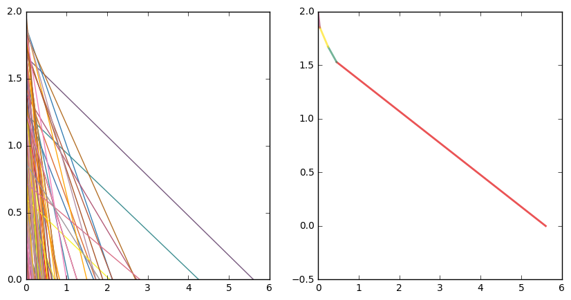
Single Layer Example

import champ
import matplotlib.pyplot as plt


#generate random coefficent matrices
coeffs=champ.get_random_halfspaces(100,dim=2)
ind_2_dom=champ.get_intersection(coeffs)

plt.close()
f,axarray=plt.subplots(1,2,figsize=(10,5))
champ.plot_line_coefficients(coeffs,axarray[0])
champ.plot_single_layer_modularity(ind_2_dom,axarray[1])
plt.show()

Output [1] :

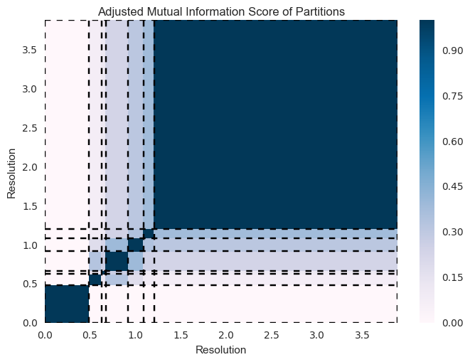
Heatmap Example

In most cases CHAMP reduces the number of considerable parttions drastically. So much so that it is feasible to calculate the similarity between all pairs of paritions and visualize them ordered by their domains. The easier way to do this is to wrap the input partitions into a louvain_ext.PartitionEnsemble object . Creation of the PartitionEnsemble object automatically applies CHAMP and allows access to the dominant partitions.

champ.plot_similarity_heatmap_single_layer(partitions, index_2_domain, partitions_other=None, index_2_dom_other=None, sim_mat=None, ax=None, cmap=None, title=None)

Parameters:

• partitions –
• index_2_domain –
• sim_mat –
• ax (Matplotlib.Axes) – Axes to draw the figure on. New figure created if not supplied.
• cmap (Matplotlib.colors.Colormap) – Color mapping. Default is plasma
• title (boolean or string) – True if add generic title, or string of title to add

Returns:

axis drawn on , computed similarity matrix

Return type:

matplolib.Axes,np.array

import champ
from champ import louvain_ext
import igraph as ig
import numpy as np
import matplotlib.pyplot as plt

np.random.seed(0)
test_graph=ig.Graph.Random_Bipartite(n1=100,n2=100,p=.1)

#parallelized wrapper
ensemb=louvain_ext.parallel_louvain(test_graph,
                                  numruns=300,start=0,fin=4,
                                  numprocesses=2,
                                  progress=True)



plt.close()
a,nmi=champ.plot_similarity_heatmap_single_layer(ensemb.partitions,ensemb.ind2doms,title=True)
plt.show()

Output [1] :

Run 0 at gamma = 0.000. Return time: 0.0275

Run 100 at gamma = 1.333. Return time: 0.0716

Run 200 at gamma = 2.667. Return time: 0.0717

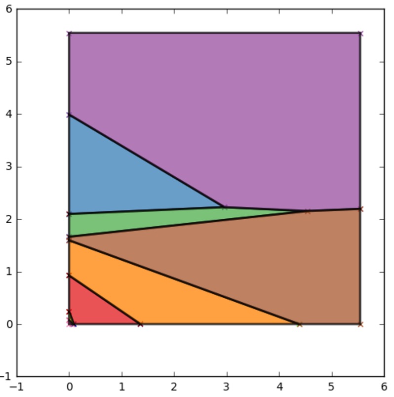
Multiayer Plots

In the multilayer case, each domain is a convex ploygon in the \((\gamma,\omega)\) plane.

champ.plot_2d_domains(ind_2_domains, ax=None, col=None, close=False, widths=None, label=False)

Parameters:

• ind_2_domains –
• ax –
• col –
• close –
• widths –
• label –

Returns:

Multilayer Example

import champ
import matplotlib.pyplot as plt

#generate random coefficent matrices
coeffs=champ.get_random_halfspaces(100,dim=3)
ind_2_dom=champ.get_intersection(coeffs)


ax=champ.plot_2d_domains(ind_2_dom)
plt.show()

Output [1] :

• Index
• Search Page

[1]	(1, 2, 3) Note that actual output might differ due to random seeding.