Louvain Parallel Extension
CHAMP can be used with partitions generated by any community detection algorithm. One of the most popular and fast algorithms is known as Louvain [1] . We provide an extension to the python package developed by Vincent Traag, louvain_igraph [2] to run Louvain in parallel, while calculating the coefficients necessary for CHAMP. Currently, this extension only support single-layer network. The random seed is set within each parallel process to ensure that the results are stochastic over each run. In general this is desireable because Louvain uses a greedy optimization schema that finds local optima.
-
champ.parallel_louvain(graph, start=0, fin=1, numruns=200, maxpt=None, numprocesses=None, attribute=None, weight=None, node_subset=None, progress=None)[source]¶ Generates arguments for parallel function call of louvain on graph
Parameters: - graph – igraph object to run Louvain on
- start – beginning of range of resolution parameter \(\gamma\) . Default is 0.
- fin – end of range of resolution parameter \(\gamma\). Default is 1.
- numruns – number of intervals to divide resolution parameter, \(\gamma\) range into
- maxpt (int) – Cutoff off resolution for domains when applying CHAMP. Default is None
- numprocesses – the number of processes to spawn. Default is number of CPUs.
- weight – If True will use ‘weight’ attribute of edges in runnning Louvain and calculating modularity.
- node_subset – Optionally list of indices or attributes of nodes to keep while partitioning
- attribute – Which attribute to filter on if node_subset is supplied. If None, node subset is assumed to be node indices.
- progress – Print progress in parallel execution every n iterations.
Returns: PartitionEnsemble of all partitions identified.
We also have created a convenient class for managing and merging groups of partitions called champ.PartitionEnsemble . This class stores the partitions in membership vector form ( i.e. a list of N community assignments), as well as the coefficients for the partitions. As part of its constructor, the PartitionEnsemble applies CHAMP to all of its partitions, and stores the domains of dominance.
-
class
champ.PartitionEnsemble(graph=None, interlayer_graph=None, layer_vec=None, listofparts=None, name='unnamed_graph', maxpt=None, min_com_size=5)[source]¶ Group of partitions of a graph stored in membership vector format
The attribute for each partition is stored in an array and can be indexed
Variables: - graph – The graph associated with this PartitionEnsemble. Each ensemble can only have a single graph and the nodes on the graph must be orded the same as each of the membership vectors. In the case of mutlilayer, graph should be a sinlge igraph containing all of the interlayer connections.
- interlayer_graph – For multilayer graph. igraph.Graph that contains all of the interlayer connections
- partitions – of membership vectors for each partition. If h5py is set this is a dummy variable that allows access to the file, but never actually hold the array of parititons.
- int_edges – Number of edges internal to the communities
- exp_edges – Number of expected edges (based on configuration model)
- resoltions – If partitions were idenitfied with Louvain, what resolution were they identified at (otherwise None)
- orig_mods – Modularity of partition at the resolution it was identified at if Louvain was used (otherwise None).
- numparts – number of partitions
- ind2doms – Maps index of dominant partitions to boundary points of their dominant domains
- ncoms – List with number of communities for each partition
- min_com_size – How many nodes must be in a community for it to count towards the number of communities. This eliminates very small or unstable communities. Default is 5
- unique_partition_indices – The indices of the paritions that represent unique coefficients. This will be a subset of all the partitions.
- hdf5_file – Current hdf5_file. If not None, this serves as the default location for loading and writing partitions to, as well as the default location for saving.
- twin_partitions – We define twin partitions as those that have the same coefficients, but are actually different partitions. This and the unique_partition_indices are only calculated on demand which can take some time.
Partition Ensemble Example
We use igraph to generate a random ER graph, call louvain in parallel, and apply CHAMP to the ensemble. This example took approximately 1 minute to run on 2 cores. We can use the PartitionEnsemble object to check whether all of the coefficients are unique, and to check whether all of the partitions themselve are unique (it is possible for two unique partitions to give rise to the same coefficients).
import champ
import igraph as ig
import tempfile
import numpy as np
import matplotlib.pyplot as plt
np.random.seed(0)
test_graph=ig.Graph.Erdos_Renyi(500,p=.05)
#Create temporary file for calling louvain
tfile=tempfile.NamedTemporaryFile('wb')
test_graph.write_graphmlz(tfile.name)
# non-parallelized wrapper
ens1=champ.run_louvain(tfile.name,nruns=5,gamma=1)
# parallelized wrapper
test_graph2=ig.Graph.Random_Bipartite(n1=100,n2=100,p=.1)
ens2=champ.parallel_louvain(test_graph2,
numruns=1000,start=0,fin=4,maxpt=4,
numprocesses=2,
progress=True)
print ("%d of %d partitions are unique"%(len(ens2.unique_partition_indices),ens2.numparts))
print ("%d of %d partitions after application of CHAMP"%(len(ens2.ind2doms),ens2.numparts))
print ("Number of twin sets:")
print (ens2.twin_partitions)
#plot both of these
plt.close()
f,a=plt.subplots(1,3,figsize=(21,7))
a1,a2,a3=a
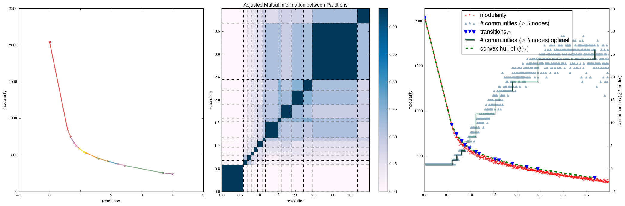
champ.plot_single_layer_modularity_domains(ens2.ind2doms,ax=a1,labels=True)
champ.plot_similarity_heatmap_single_layer(ens2.partitions,ens2.ind2doms,ax=a2,title=True)
#PartitionEnsemble has method to plot downsampled summary of all partitions
#with optmal transitions and number of communities overlayed.
ens2.plot_modularity_mapping(ax=a3,no_tex=False)
plt.tight_layout()
plt.show()
Output:
We see that there are a number of identical partitions here, there are no twin partitions . That is different partitions with the same coefficents.
-
PartitionEnsemble.apply_CHAMP(subset=None, maxpt=None)[source]¶ Apply CHAMP to the partition ensemble.
Parameters: - maxpt (int) – maximum domain threshhold for included partition. I.e partitions with a domain greater than maxpt will not be included in pruned set
- subset – subset of partitions to apply CHAMP to. This is useful in merging two sets because we only need to apply champ to the combination of the two
-
PartitionEnsemble.plot_modularity_mapping(ax=None, downsample=2000, champ_only=False, legend=True, no_tex=True)[source]¶ Plot a scatter of the original modularity vs gamma with the modularity envelope super imposed. Along with communities vs \(\gamma\) on a twin axis. If no orig_mod values are stored in the ensemble, just the modularity envelope is plotted. Depending on the backend used to render plot the latex in the labels can cause error. If you are getting RunTime errors when showing or saving the plot, try setting no_tex=True
Parameters: - ax (matplotlib.Axes) – axes to draw the figure on.
- champ_only (bool) – Only plot the modularity envelop represented by the CHAMP identified subset.
- downsample (int) – for large number of runs, we down sample the scatter for the number of communities and the original partition set. Default is 2000 randomly selected partitions.
- legend (bool) – Add legend to the figure. Default is true
- no_tex (bool) – Use latex in the legends. Default is true. If error is thrown on plotting try setting this to false.
Returns: axes drawn upon
Return type: matplotlib.Axes
-
PartitionEnsemble.get_unique_partition_indices(reindex=True)[source]¶ This returns the indices for the partitions who are unique. This could be larger than the indices for the unique coeficient since multiple partitions can give rise to the same coefficient. In practice this has been very rare. This function can take sometime for larger network with many partitions since it reindex the partitions labels to ensure they aren’t permutations of each other.
Parameters: reindex – if True, will reindex partitions that it is comparing to ensure they are unique under permutation. Returns: list of twin partition (can be empty), list of indicies of unique partitions. Return type: list,np.array
-
PartitionEnsemble.twin_partitions¶ We define twin partitions as those that have the same coefficients but are different partitions. To find these we look for the diffence in the partitions with the same coefficients.
Returns: List of groups of the indices of partitions that have the same coefficient but are non-identical. Return type: list of list (possibly empty if no twins)
Creating and Managing Large Partition Sets
For large sets of partitions on larger networks, loading the entire set of partitions each time you want to access the data can take a fair amount of time. Having to load all of the partitions defeats the purpose of using CHAMP to find the optimal subset. As such we have equiped champ.louvain_ext.PartitionEnsemble objects with the ability to write to and access hdf5 files. Instead of loading the entire set of partitions each time, only the coefficients, the domains of dominance, the underlying graph information is loaded, vastly reducing the
loading time and the memory required for large numbers of runs. Each individual partitions ( or all partitions at once) can be access from file only if needed, as the example below illustrates:
Saving and Loading PartitionEnsembles
import champ
import igraph as ig
import numpy as np

np.random.seed(0)
test_graph=ig.Graph.Erdos_Renyi(n=200,p=.1)
times={}
run_nums=[100]

#saving ensemble
ensemble=champ.parallel_louvain(test_graph,numprocesses=2,numruns=200,start=0,fin=4,maxpt=4,progress=False)
print "Ensemble 1, Optimal subset is %d of %d partitions"%(len(ensemble.ind2doms),ensemble.numparts)
ensemble.save("ensemble1.hdf5",hdf5=True)

#openning created file
ensemble2=champ.PartitionEnsemble().open("ensemble1.hdf5")
#partitions is an internal class the handles access
print ensemble2.partitions
#When sliced a numpy.array is returned
print "ensemble2.partitions[38,:10]:\n\t",ensemble2.partitions[38:40,:10]

#You can still add partitions as normal.  These are automatically
#added to the hdf5 file
ensemble2add=champ.parallel_louvain(test_graph,numprocesses=2,numruns=100,start=0,fin=4,maxpt=4,progress=False)
ensemble2.add_partitions(ensemble2add.get_partition_dictionary())
print "ensemble 2 has %d of %d partitions dominant"  %(len(ensemble2.ind2doms),ensemble2.numparts)

#When open is called, the created EnsemblePartition assumes all
#the state variables of saved EnsemblePartition, including default save file.
#If save() is called, it will overwrite the old ensemble file
print "ensemble2 default hdf5 file: ",ensemble2.hdf5_file
Output:
You can see with the above example that CHAMP is reapplied everytime new partitions are added to the PartitionEnsemble instance. In addition, whole PartitionEnsemble objects can be merged together in a similar fashion. You can either have a new PartitionEnsemble generated, containing the contents of both the inputs. Or one partition can be merged into the other one. It automatically uses the larger of the two to merge into. In addition, if either PartitionEnsemble has an associated hdf5 file, the merger will just expand the contents of the file and keep the same PartitionEnsemble object.
-
PartitionEnsemble.add_partitions(partitions, maxpt=None)[source]¶ Add additional partitions to the PartitionEnsemble object. Also adds the number of communities for each. In the case where PartitionEnsemble was openned from a file, we just appended these and the other values onto each of the files. Partitions are not kept in object, however the other partitions values are.
Parameters: partitions (dict,list) – list of partitions to add to the PartitionEnsemble
-
PartitionEnsemble.hdf5_file¶ Default location for saving/loading PartitionEnsemble if hdf5 format is used. When this is set it will automatically resave the PartitionEnsemble into the file specified.
-
PartitionEnsemble.save(filename=None, dir='.', hdf5=True, compress=9)[source]¶ Use pickle or h5py to store representation of PartitionEnsemble in compressed file. When called if object has an assocated hdf5_file, this is the default file written to. Otherwise objected is stored using pickle.
Parameters: - filename – name of file to write to. Default is created from name of ParititonEnsemble: “%s_PartEnsemble_%d” %(self.name,self.numparts)
- hdf5 (bool) – save the PartitionEnsemble object as a hdf5 file. This is very useful for larger partition sets, especially when you only need to work with the optimal subset. If object has hdf5_file attribute saved this becomes the default
- compress (int [0,9]) – Level of compression for partitions in hdf5 file. With less compression, files take longer to write but take up more space. 9 is default.
- dir (str) – directory to save graph in. relative or absolute path. default is working dir.
-
PartitionEnsemble.save_graph(filename=None, dir='.', intra=True)[source]¶ Save a copy of the graph with each of the optimal partitions stored as vertex attributes in graphml compressed format. Each partition is attribute names part_gamma where gamma is the beginning of the partitions domain of dominance. Note that this is seperate from the information about the graph that is saved within the hdf5 file along side the partions.
Parameters: - filename – name of file to write out to. Default is self.name.graphml.gz or :type filename: str
- dir (str) – directory to save graph in. relative or absolute path. default is working dir.
Merging PartitionEnsembles
import champ
import igraph as ig
import numpy as np

np.random.seed(0)
test_graph=ig.Graph.Erdos_Renyi(n=200,p=.1)
times={}
run_nums=[100]

ensemble=champ.parallel_louvain(test_graph,numprocesses=2,numruns=200,start=0,fin=4,maxpt=4,progress=False)
print "Ensemble 1, Optimal subset is %d of %d partitions"%(len(ensemble.ind2doms),ensemble.numparts)
ensemble.save("ensemble1.hdf5",hdf5=True)

ensemble2=champ.parallel_louvain(test_graph,numprocesses=2,numruns=200,start=0,fin=4,maxpt=4,progress=False)
print "Ensemble 2, Optimal subset is %d of %d partitions"%(len(ensemble2.ind2doms),ensemble2.numparts)
ensemble2.save("ensemble2.hdf5",hdf5=True)

#Esembles can be merged as follows:

#Create new PartitionEnsemble from scratch
ensemble3=ensemble.merge_ensemble(ensemble2,new=True)
print "Ensemble 3, Optimal subset is %d of %d partitions"%(len(ensemble3.ind2doms),ensemble3.numparts)

#Use largest of the 2 PartitionEnsembles being merged  and modify
ensemble4=ensemble.merge_ensemble(ensemble3,new=False)
print "Ensemble 4, Optimal subset is %d of %d partitions"%(len(ensemble4.ind2doms),ensemble4.numparts)
print "ensemble4 is ensemble3: ",ensemble4 is ensemble3
Output:
-
PartitionEnsemble.merge_ensemble(otherEnsemble, new=True)[source]¶ Combine to PartitionEnsembles. Checks for concordance in the number of vertices. Assumes that internal ordering on the graph nodes for each is the same.
Parameters: - otherEnsemble – otherEnsemble to merge
- new (bool) – create a new PartitionEnsemble object? Otherwise partitions will be loaded into the one of the original partition ensemble objects (the one with more partitions in the first place).
Returns: PartitionEnsemble reference with merged set of partitions
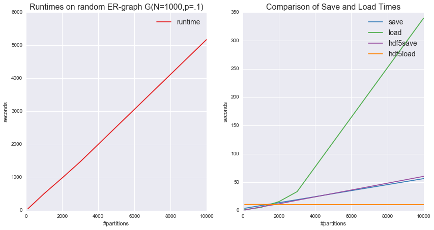
Improvement with HDF5 saving and loading
The following example gives a sense of when it is beneficial to save as HDF5 and general runtimes for parallelized Louvain. We also found that the overhead is dependent on the size of the graph as well, so that for larger graphs with a lower number of partitions, the read/write time on HDF5 can be greater. Total runtime was about 2.5 hours on 10 CPUs.
import champ
import matplotlib.pyplot as plt
import seaborn as sbn
import numpy as np
import pandas as pd
import igraph as ig
from time import time

np.random.seed(0)
test_graph=ig.Graph.Erdos_Renyi(n=1000,p=.1)

times={}
run_nums=[100,1000,2000,3000,10000]

for nrun in run_nums :
    rtimes=[]
    t=time()
    ens=champ.parallel_louvain(test_graph,numprocesses=10,numruns=nrun,start=0,fin=4,maxpt=4,progress=False)
    ens.name='name'
    rtimes.append(time()-t)

    #normal save (gzip)
    print "CHAMP running time %d runs: %.3f" %(nrun,rtimes[-1])
    t=time()
    ens.save()
    rtimes.append(time()-t)
    t=time()

    #normal open
    t=time()
    newens=champ.PartitionEnsemble().open("name_PartEnsemble_%d.gz"%nrun)
    rtimes.append(time()-t)
    t=time()

    #save with h5py
    t=time()
    ens.save(hdf5=True)
    rtimes.append(time()-t)
    t=time()

    #open with hdf5 format
    t=time()
    newes=champ.PartitionEnsemble().open("name_PartEnsemble_%d.hdf5"%nrun)
    rtimes.append(time()-t)
    times[nrun]=rtimes

tab=pd.DataFrame(times,columns=run_nums,index=['runtime','save','load','hdf5save','hdf5load'])
colors=sbn.color_palette('Set1',n_colors=tab.shape[0])
plt.close()
f,(a1,a2)=plt.subplots(1,2,figsize=(14,7))
for i,ind in enumerate(tab.index.values):
    if ind=='runtime':
        a1.plot(tab.columns,tab.loc[ind,:],label=ind,color=colors[i])
    else:
        a2.plot(tab.columns,tab.loc[ind,:],label=ind,color=colors[i])

a1.set_xlabel("#partitions")
a1.set_ylabel("seconds")
a2.set_xlabel("#partitions")
a2.set_ylabel("seconds")

a2.set_title("Comparison of Save and Load Times",fontsize=16)
a1.set_title("Runtimes on random ER-graph G(N=1000,p=.1)",fontsize=16)
a1.legend(fontsize=14)
a2.legend(fontsize=14)
plt.show()
Output: